Basic Usage
API
The package follows scikit-learn API, with a minor adaptation to work with time and event data (y as a numpy structured array of times and events). .predict() returns a dataframe where each column is a time window and values represent the probability of survival before or exactly at the time window.
# importing dataset from pycox package
from pycox.datasets import metabric

# importing model and utils from xgbse
from xgbse import XGBSEKaplanNeighbors
from xgbse.converters import convert_to_structured

# getting data
df = metabric.read_df()

# splitting to X, y format
X = df.drop(['duration', 'event'], axis=1)
y = convert_to_structured(df['duration'], df['event'])

# fitting xgbse model
xgbse_model = XGBSEKaplanNeighbors(n_neighbors=50)
xgbse_model.fit(X, y)

# predicting
event_probs = xgbse_model.predict(X)
event_probs.head()| index | 15 | 30 | 45 | 60 | 75 | 90 | 105 | 120 | 135 | 150 | 165 | 180 | 195 | 210 | 225 | 240 | 255 | 270 | 285 |
|---|---|---|---|---|---|---|---|---|---|---|---|---|---|---|---|---|---|---|---|
| 0 | 0.98 | 0.87 | 0.81 | 0.74 | 0.71 | 0.66 | 0.53 | 0.47 | 0.42 | 0.4 | 0.3 | 0.25 | 0.21 | 0.16 | 0.12 | 0.098 | 0.085 | 0.062 | 0.054 |
| 1 | 0.99 | 0.89 | 0.79 | 0.7 | 0.64 | 0.58 | 0.53 | 0.46 | 0.42 | 0.39 | 0.33 | 0.31 | 0.3 | 0.24 | 0.21 | 0.18 | 0.16 | 0.11 | 0.095 |
| 2 | 0.94 | 0.78 | 0.63 | 0.57 | 0.54 | 0.49 | 0.44 | 0.37 | 0.34 | 0.32 | 0.26 | 0.23 | 0.21 | 0.16 | 0.13 | 0.11 | 0.098 | 0.072 | 0.062 |
| 3 | 0.99 | 0.95 | 0.93 | 0.88 | 0.84 | 0.81 | 0.73 | 0.67 | 0.57 | 0.52 | 0.45 | 0.37 | 0.33 | 0.28 | 0.23 | 0.19 | 0.16 | 0.12 | 0.1 |
| 4 | 0.98 | 0.92 | 0.82 | 0.77 | 0.72 | 0.68 | 0.63 | 0.6 | 0.57 | 0.55 | 0.51 | 0.48 | 0.45 | 0.42 | 0.38 | 0.33 | 0.3 | 0.22 | 0.2 |
You can also get interval predictions (probability of failing exactly at each time window) using return_interval_probs:
# point predictions
interval_probs = xgbse_model.predict(X_valid, return_interval_probs=True)
interval_probs.head()| index | 15 | 30 | 45 | 60 | 75 | 90 | 105 | 120 | 135 | 150 | 165 | 180 | 195 | 210 | 225 | 240 | 255 | 270 | 285 |
|---|---|---|---|---|---|---|---|---|---|---|---|---|---|---|---|---|---|---|---|
| 0 | 0.024 | 0.1 | 0.058 | 0.07 | 0.034 | 0.05 | 0.12 | 0.061 | 0.049 | 0.026 | 0.096 | 0.049 | 0.039 | 0.056 | 0.04 | 0.02 | 0.013 | 0.023 | 0.0078 |
| 1 | 0.014 | 0.097 | 0.098 | 0.093 | 0.052 | 0.065 | 0.054 | 0.068 | 0.034 | 0.038 | 0.053 | 0.019 | 0.018 | 0.052 | 0.038 | 0.027 | 0.018 | 0.05 | 0.015 |
| 2 | 0.06 | 0.16 | 0.15 | 0.054 | 0.033 | 0.053 | 0.046 | 0.073 | 0.032 | 0.014 | 0.06 | 0.03 | 0.017 | 0.055 | 0.031 | 0.016 | 0.014 | 0.027 | 0.0097 |
| 3 | 0.011 | 0.034 | 0.021 | 0.053 | 0.038 | 0.038 | 0.08 | 0.052 | 0.1 | 0.049 | 0.075 | 0.079 | 0.037 | 0.052 | 0.053 | 0.041 | 0.026 | 0.04 | 0.017 |
| 4 | 0.016 | 0.067 | 0.099 | 0.046 | 0.05 | 0.042 | 0.051 | 0.028 | 0.03 | 0.018 | 0.048 | 0.022 | 0.029 | 0.038 | 0.035 | 0.047 | 0.031 | 0.08 | 0.027 |
Survival curves and confidence intervals
XBGSEKaplanTree and XBGSEKaplanNeighbors support estimation of survival curves and confidence intervals via the Exponential Greenwood formula out-of-the-box via the return_ci argument:
# fitting xgbse model
xgbse_model = XGBSEKaplanNeighbors(n_neighbors=50)
xgbse_model.fit(X_train, y_train, time_bins=TIME_BINS)

# predicting
mean, upper_ci, lower_ci = xgbse_model.predict(X_valid, return_ci=True)

# plotting CIs
plot_ci(mean, upper_ci, lower_ci)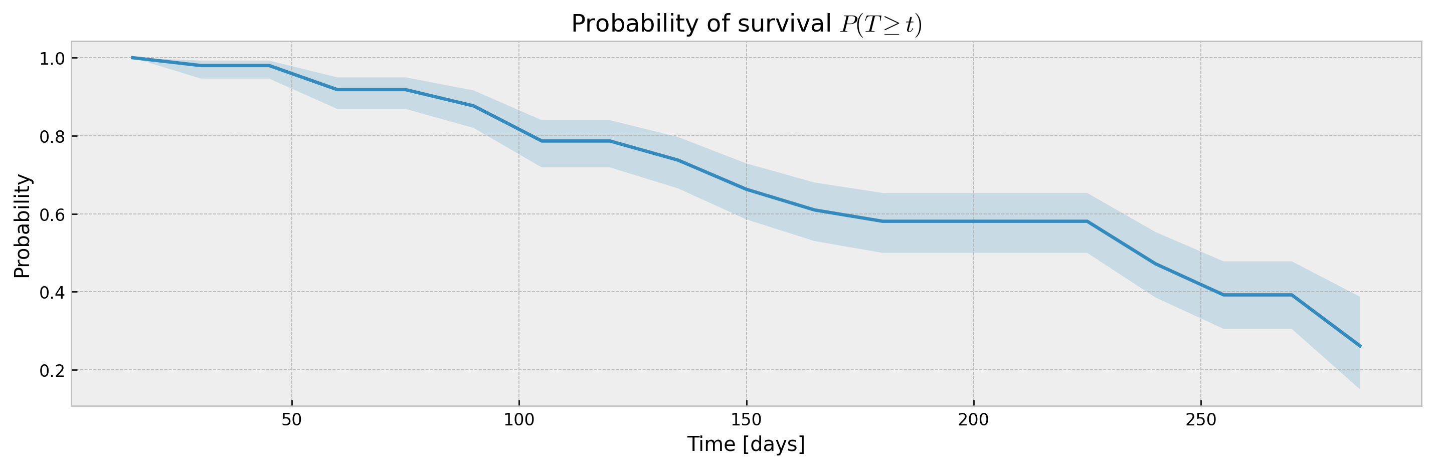
XGBSEDebiasedBCE does not support estimation of confidence intervals out-of-the-box, but we provide the XGBSEBootstrapEstimator to get non-parametric confidence intervals. As the stacked logistic regressions are trained with more samples (in comparison to neighbor-sets in XGBSEKaplanNeighbors), confidence intervals are more concentrated:
# base model as BCE
base_model = XGBSEDebiasedBCE(PARAMS_XGB_AFT, PARAMS_LR)

# bootstrap meta estimator
bootstrap_estimator = XGBSEBootstrapEstimator(base_model, n_estimators=20)

# fitting the meta estimator
bootstrap_estimator.fit(
    X_train,
    y_train,
    validation_data=(X_valid, y_valid),
    early_stopping_rounds=10,
    time_bins=TIME_BINS,
)

# predicting
mean, upper_ci, lower_ci = bootstrap_estimator.predict(X_valid, return_ci=True)

# plotting CIs
plot_ci(mean, upper_ci, lower_ci)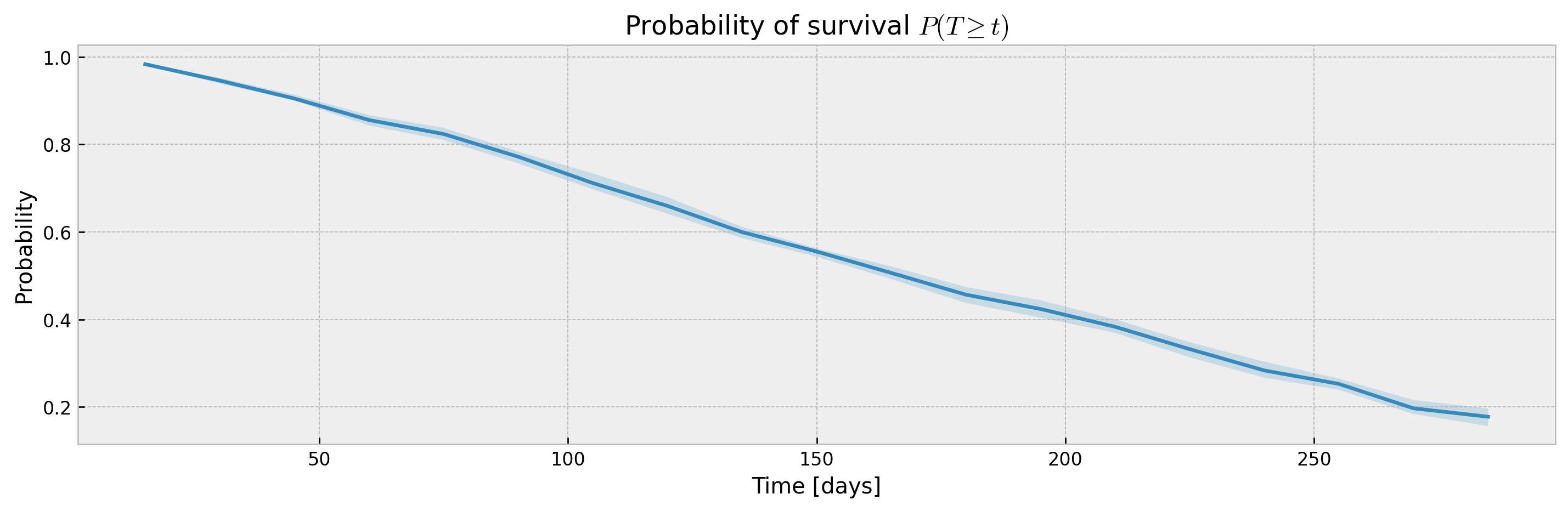
The bootstrap abstraction can be used for XBGSEKaplanTree and XBGSEKaplanNeighbors as well, however, the confidence interval will be estimated via bootstrap only (not Exponential Greenwood formula):
# base model
base_model = XGBSEKaplanTree(PARAMS_TREE)

# bootstrap meta estimator
bootstrap_estimator = XGBSEBootstrapEstimator(base_model, n_estimators=100)

# fitting the meta estimator
bootstrap_estimator.fit(
    X_train,
    y_train,
    time_bins=TIME_BINS,
)

# predicting
mean, upper_ci, lower_ci = bootstrap_estimator.predict(X_valid, return_ci=True)

# plotting CIs
plot_ci(mean, upper_ci, lower_ci)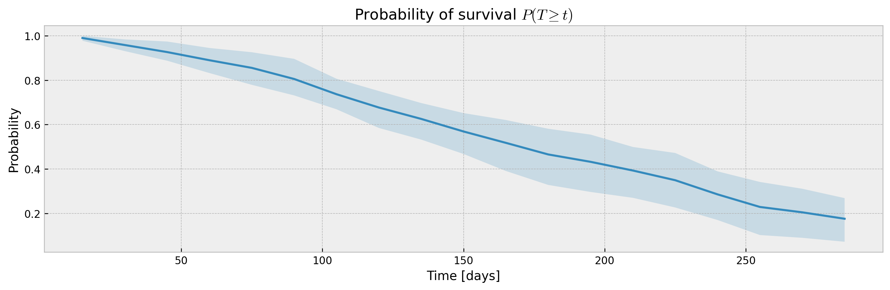
With a sufficiently large n_estimators, interval width shouldn't be much different, with the added benefit of model stability and improved accuracy. Addittionaly, XGBSEBootstrapEstimator allows building confidence intervals for interval probabilities (which is not supported for Exponential Greenwood):
# predicting
mean, upper_ci, lower_ci = bootstrap_estimator.predict(
    X_valid,
    return_ci=True,
    return_interval_probs=True
)

# plotting CIs
plot_ci(mean, upper_ci, lower_ci)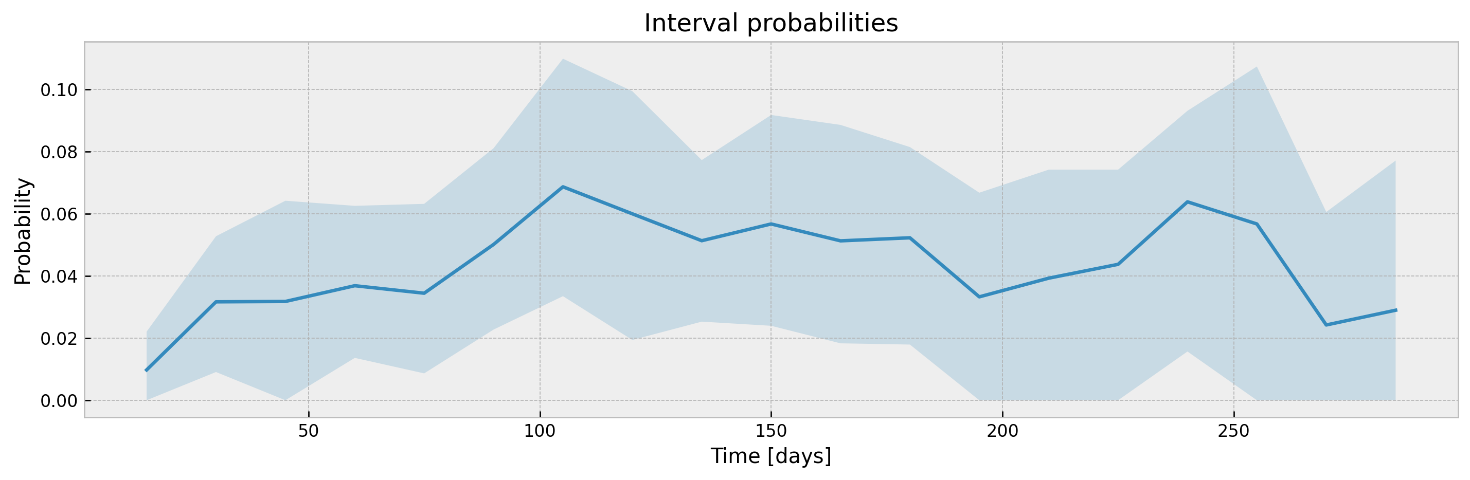
The parameter ci_width controls the width of the confidence interval. For XGBSEKaplanTree it should be passed at .fit(), as KM curves are pre-calculated for each leaf at fit time to avoid storing training data.
# fitting xgbse model
xgbse_model = XGBSEKaplanTree(PARAMS_TREE)
xgbse_model.fit(X_train, y_train, time_bins=TIME_BINS, ci_width=0.99)

# predicting
mean, upper_ci, lower_ci = xgbse_model.predict(X_valid, return_ci=True)

# plotting CIs
plot_ci(mean, upper_ci, lower_ci)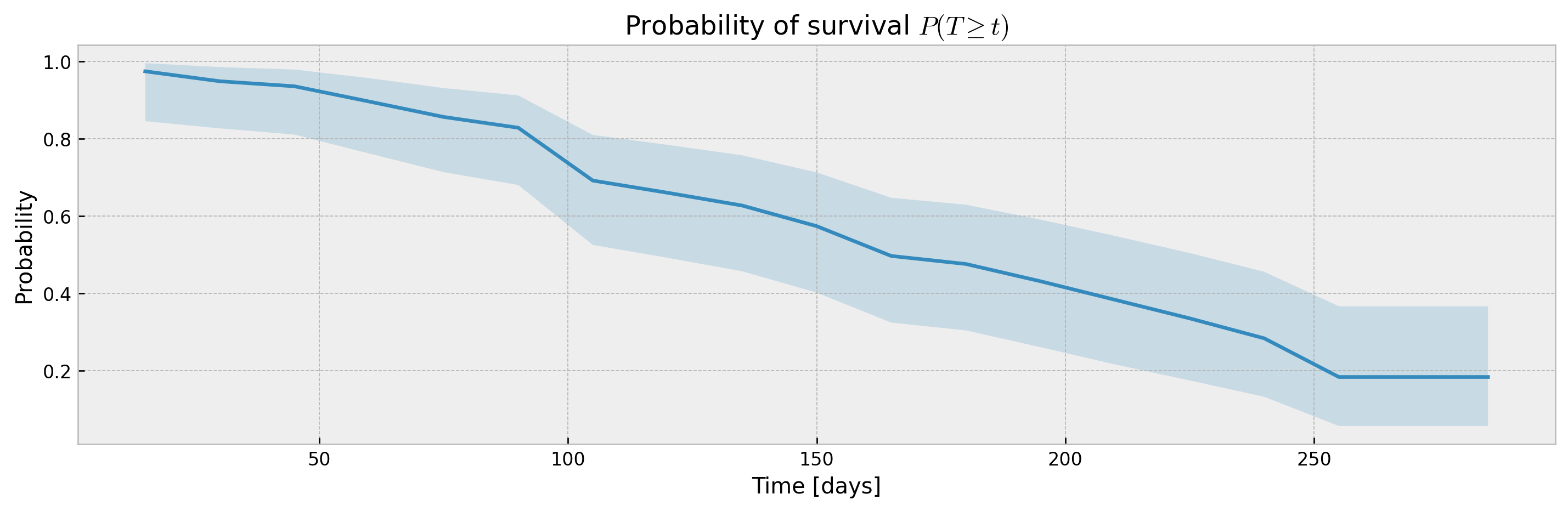
For other models (XGBSEKaplanNeighbors and XGBSEBootstrapEstimator) it should be passed at .predict().
# base model
model = XGBSEKaplanNeighbors(PARAMS_XGB_AFT, N_NEIGHBORS)

# fitting the meta estimator
model.fit(
    X_train, y_train,
    validation_data = (X_valid, y_valid),
    early_stopping_rounds=10,
    time_bins=TIME_BINS
)

# predicting
mean, upper_ci, lower_ci = model.predict(X_valid, return_ci=True, ci_width=0.99)

# plotting CIs
plot_ci(mean, upper_ci, lower_ci)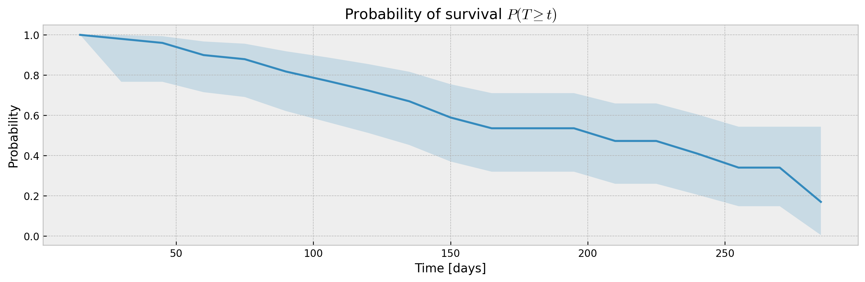
Early stopping
A simple interface to xgboost early stopping is provided.
# splitting between train, and validation
(X_train, X_valid,
 y_train, y_valid) = \
train_test_split(X, y, test_size=0.2, random_state=42)

# fitting with early stopping
xgb_model = XGBSEDebiasedBCE()
xgb_model.fit(
    X_train,
    y_train,
    validation_data=(X_valid, y_valid),
    early_stopping_rounds=10,
    verbose_eval=50
)
[0] validation-aft-nloglik:16.86713
Will train until validation-aft-nloglik hasn't improved in 10 rounds.
[50] validation-aft-nloglik:3.64540
[100] validation-aft-nloglik:3.53679
[150] validation-aft-nloglik:3.53207
Stopping. Best iteration:
[174] validation-aft-nloglik:3.53004Explainability through prototypes
xgbse also provides explainability through prototypes, searching the embedding for neighbors. The idea is to explain model predictions with real samples, providing solid ground to justify them (see [8]). The method .get_neighbors() searches for the n_neighbors nearest neighbors in index_data for each sample in query_data:
neighbors = xgb_model.get_neighbors(
    query_data=X_valid,
    index_data=X_train,
    n_neighbors=10
)
neighbors.head(5)| index | neighbor_1 | neighbor_2 | neighbor_3 | neighbor_4 | neighbor_5 | neighbor_6 | neighbor_7 | neighbor_8 | neighbor_9 | neighbor_10 |
|---|---|---|---|---|---|---|---|---|---|---|
| 1225 | 1151 | 1513 | 1200 | 146 | 215 | 452 | 1284 | 1127 | 1895 | 257 |
| 111 | 1897 | 1090 | 1743 | 1224 | 892 | 1695 | 1624 | 1546 | 1418 | 4 |
| 554 | 9 | 627 | 1257 | 1460 | 1031 | 1575 | 1557 | 440 | 1236 | 858 |
| 526 | 726 | 1042 | 177 | 1640 | 242 | 1529 | 234 | 1800 | 399 | 1431 |
| 1313 | 205 | 1738 | 599 | 954 | 1694 | 1715 | 1651 | 828 | 541 | 992 |
This way, we can inspect neighbors of a given sample to try to explain predictions. For instance, we can choose a reference and check that its neighbors actually are very similar as a sanity check:
i = 0

reference = X_valid.iloc[i]
reference.name = 'reference'
train_neighs = X_train.loc[neighbors.iloc[i]]

pd.concat([reference.to_frame().T, train_neighs])| index | x0 | x1 | x2 | x3 | x4 | x5 | x6 | x7 | x8 |
|---|---|---|---|---|---|---|---|---|---|
| reference | 5.7 | 5.7 | 11 | 5.6 | 1 | 1 | 0 | 1 | 86 |
| 1151 | 5.8 | 5.9 | 11 | 5.5 | 1 | 1 | 0 | 1 | 82 |
| 1513 | 5.5 | 5.5 | 11 | 5.6 | 1 | 1 | 0 | 1 | 79 |
| 1200 | 5.7 | 6 | 11 | 5.6 | 1 | 1 | 0 | 1 | 76 |
| 146 | 5.9 | 5.9 | 11 | 5.5 | 0 | 1 | 0 | 1 | 75 |
| 215 | 5.8 | 5.5 | 11 | 5.4 | 1 | 1 | 0 | 1 | 78 |
| 452 | 5.7 | 5.7 | 12 | 5.5 | 0 | 0 | 0 | 1 | 76 |
| 1284 | 5.6 | 6.2 | 11 | 5.6 | 1 | 0 | 0 | 1 | 79 |
| 1127 | 5.5 | 5.1 | 11 | 5.5 | 1 | 1 | 0 | 1 | 86 |
| 1895 | 5.5 | 5.4 | 10 | 5.5 | 1 | 1 | 0 | 1 | 85 |
| 257 | 5.7 | 6 | 9.6 | 5.6 | 1 | 1 | 0 | 1 | 76 |
We also can compare the Kaplan-Meier curve estimated from the neighbors to the actual model prediction, checking that it is inside the confidence interval:
from xgbse.non_parametric import calculate_kaplan_vectorized

mean, high, low = calculate_kaplan_vectorized(
    np.array([y['c2'][neighbors.iloc[i]]]),
    np.array([y['c1'][neighbors.iloc[i]]]),
    TIME_BINS
)

model_surv = xgb_model.predict(X_valid)

plt.figure(figsize=(12,4), dpi=120)
plt.plot(model_surv.columns, model_surv.iloc[i])
plt.plot(mean.columns, mean.iloc[0])
plt.fill_between(mean.columns, low.iloc[0], high.iloc[0], alpha=0.1, color='red')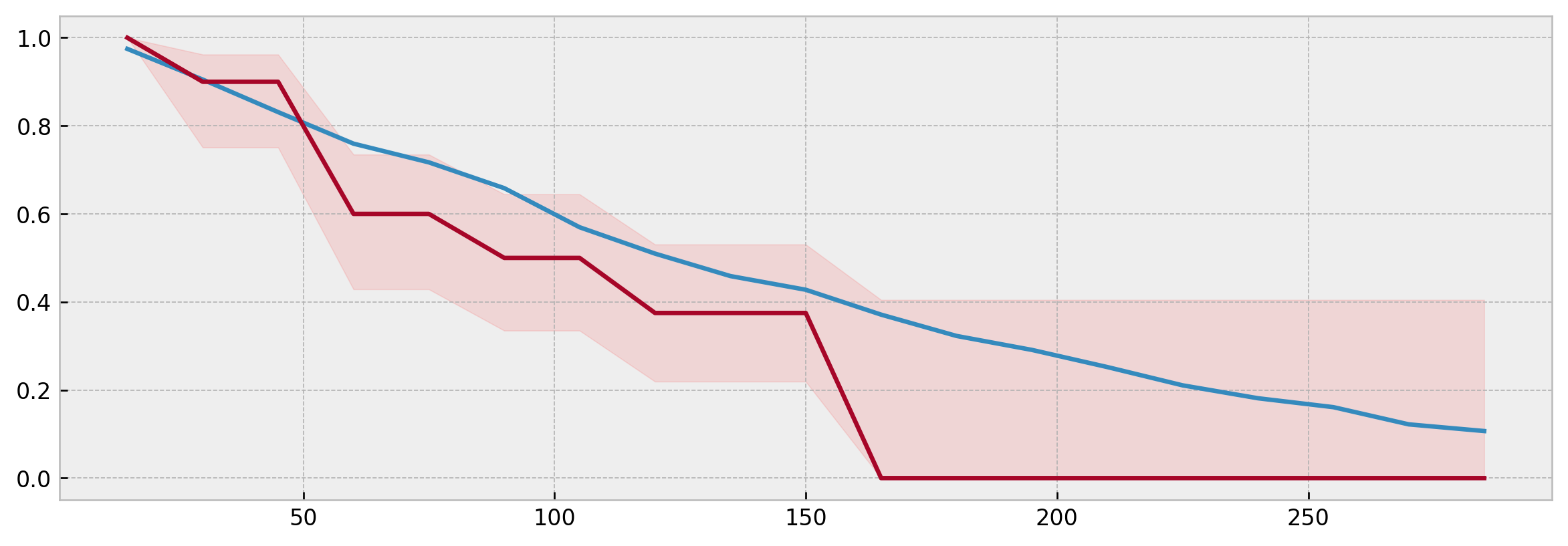
Specifically, for XBGSEKaplanNeighbors prototype predictions and model predictions should match exactly if n_neighbors is the same and query_data is equal to the training data.
Metrics
We made our own metrics submodule to make the lib self-contained. xgbse.metrics implements C-index, Brier Score and D-Calibration from [9], including adaptations to deal with censoring:
# training model
xgbse_model = XGBSEKaplanNeighbors(PARAMS_XGB_AFT, n_neighbors=30)

xgbse_model.fit(
    X_train, y_train,
    validation_data = (X_valid, y_valid),
    early_stopping_rounds=10,
    time_bins=TIME_BINS
)

# predicting
preds = xgbse_model.predict(X_valid)

# importing metrics
from xgbse.metrics import (
    concordance_index,
    approx_brier_score,
    dist_calibration_score
)

# running metrics
print(f'C-index: {concordance_index(y_valid, preds)}')
print(f'Avg. Brier Score: {approx_brier_score(y_valid, preds)}')
print(f"""D-Calibration: {dist_calibration_score(y_valid, preds) > 0.05}""")
C-index: 0.6495863029409356
Avg. Brier Score: 0.1704190044350422
D-Calibration: Truescore_func(y, y_pred, **kwargs) pattern, we can use the sklearn model selection module easily:
from sklearn.model_selection import cross_val_score
from sklearn.metrics import make_scorer

xgbse_model = XGBSEKaplanTree(PARAMS_TREE)
results = cross_val_score(xgbse_model, X, y, scoring=make_scorer(approx_brier_score))
results
array([0.17432953, 0.15907712, 0.13783666, 0.16770409, 0.16792016])Citing xgbse
To cite this repository:
@software{xgbse2020github,
  author = {Davi Vieira and Gabriel Gimenez and Guilherme Marmerola and Vitor Estima},
  title = {XGBoost Survival Embeddings: improving statistical properties of XGBoost survival analysis implementation},
  url = {http://github.com/loft-br/xgboost-survival-embeddings},
  version = {0.2.0},
  year = {2020},
}
References
[1] X. He, J. Pan, O. Jin, T. Xu, B. Liu, T. Xu, Y. Shi, A. Atallah, R. Herbrich, S. Bowers, and J. Q. Candela. Practical Lessons from Predicting Clicks on Ads at Facebook (2014). In Proceedings of the Eighth International Workshop on Data Mining for Online Advertising (ADKDD’14).
[2][Feature transformations with ensembles of trees](https://scikit-learn.org/stable/auto_examples/ensemble/plot_feature_transformation.html). Scikit-learn documentation at https://scikit-learn.org/.
[3] G. Marmerola. Calibration of probabilities for tree-based models. Personal Blog at https://gdmarmerola.github.io/.
[4] G. Marmerola. Supervised dimensionality reduction and clustering at scale with RFs with UMAP. Personal Blog at https://gdmarmerola.github.io/.
[5] C. Yu, R. Greiner, H. Lin, V. Baracos. Learning Patient-Specific Cancer Survival Distributions as a Sequence of Dependent Regressors. Advances in Neural Information Processing Systems 24 (NIPS 2011).
[6] H. Kvamme, Ø. Borgan. The Brier Score under Administrative Censoring: Problems and Solutions. arXiv preprint arXiv:1912.08581.
[7] S. Sawyer. The Greenwood and Exponential Greenwood Confidence Intervals in Survival Analysis. Handout on Washington University in St. Louis website.
[8] H. Kvamme, Ø. Borgan, and I. Scheel. Time-to-event prediction with neural networks and Cox regression. Journal of Machine Learning Research, 20(129):1–30, 2019.
[9] H. Haider, B. Hoehn, S. Davis, R. Greiner. Effective Ways to Build and Evaluate Individual Survival Distributions. Journal of Machine Learning Research 21 (2020) 1–63.